Lattice geometries

The Ising graph serves as the starting point, allowing users to load instances directly from a file and translate them into a graph with vertices numerated using linear indices. To group spins into clusters for the Potts Hamiltonian, it is necessary to map these linear spin coordinates onto the corresponding coordinates of a Potts clusters in a specific lattice geometry.

SpinGlassPEPS.jl provides tools for mapping linear indices into three lattice geometries: super-square, Pegasus, and Zephyr. For example, groups of 24 binary spins form one Potts variable on Pegasus, while Zephyr clusters contain 16 spins.

Super square lattice

The super_square_lattice geometry defines a square lattice with interactions between nearest neighbors (horizontal and vertical connections between unit cells) and next-nearest neighbors (diagonal connections). In super_square_lattice function, linear indices of spins from the Ising graph are mapped onto a 2D super square lattice coordinate system (King's lattice). Spins (denoted as black dots in the figure below) are grouped into clusters represented as red ellipses. Every spin in this cluster is indexed coresponding to the square lattice coordinate in the new graph with reduced number of variables of higher dimensions (shown on the right).

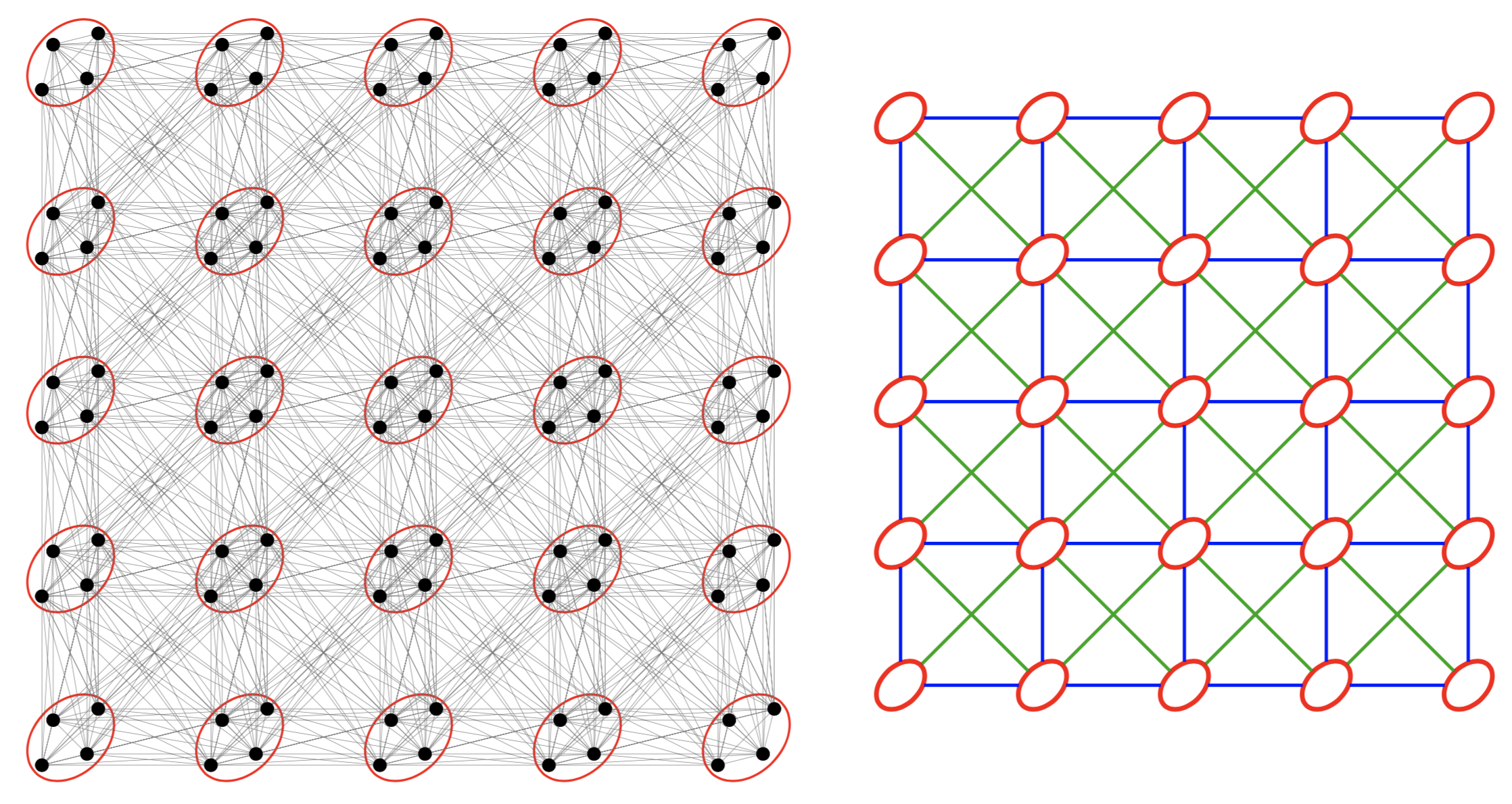
In SpinGlassPEPS.jl solver, a grid of this type can be loaded using the command super_square_lattice.

SpinGlassPEPS.SpinGlassNetworks.super_square_lattice — Function

super_square_lattice(
    size::Tuple{Int64, Int64, Int64}
) -> Dict{Int64, Tuple{Int64, Int64}}

Create a mapping from Ising graph coordinates to a super square lattice arrangement.

This function generates a mapping that relates linear Ising graph coordinates to a super square lattice arrangement. The super square lattice is defined by the size of three dimensions: (m, n, t), where m is the number of columns, n is the number of rows and t denotes the number of spins stored in the cluster.

Arguments:

size::NTuple{3, Int}: A tuple specifying the size of the super square lattice in three dimensions: (m, n, t), where m is number of columns, n number of rows and t denotes number of spins in cluster.

Returns:

coord_map::Dict: A dictionary that maps Ising graph coordinates to the corresponding lattice coordinates.

source

Below you find simple example of usage super_square_latttice function.

using SpinGlassPEPS

instance = joinpath(
    pkgdir(SpinGlassPEPS), "docs", "src", "instances", "square_diagonal", "5x5", "diagonal.txt",
)
ig = ising_graph(instance)

m = 5
n = 5
t = 4

potts_h = potts_hamiltonian(
    ig,
    cluster_assignment_rule = super_square_lattice((m, n, t))
)

println("Number of nodes in original instance: ", SpinGlassPEPS.SpinGlassNetworks.nv(ig))
println("Number of nodes in Potts Hamiltonian: ", SpinGlassPEPS.SpinGlassNetworks.nv(potts_h))

Number of nodes in original instance: 100
Number of nodes in Potts Hamiltonian: 25

Pegasus graphs

The Pegasus graph is a type of graph architecture used in quantum computing systems, particularly in the quantum annealing machines developed by D-Wave Systems. It is designed to provide a grid of qubits with specific connectivity patterns optimized for solving certain optimization problems. Futer details can be found here.

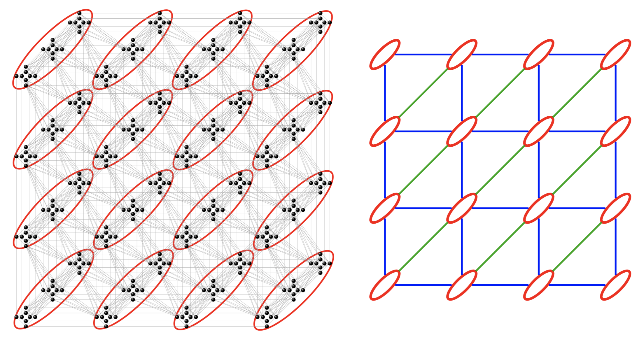
In SpinGlassPEPS.jl solver, a grid of this type can be loaded using the command pegasus_lattice.

SpinGlassPEPS.SpinGlassNetworks.pegasus_lattice — Function

pegasus_lattice(
    size::Tuple{Int64, Int64, Int64}
) -> Union{Dict{Any, Any}, Dict{Int64, Tuple{Int64, Int64, Int64}}}

Create a mapping from Ising graph coordinates to Pegasus lattice coordinates.

This function generates a mapping that relates Ising graph coordinates to Pegasus lattice coordinates based on the specified size of the Pegasus lattice in three dimensions: (m, n, t).

Arguments:

size::NTuple{3, Int}: A tuple specifying the size of the Pegasus lattice in three dimensions: (m, n, t), where m is number of columns, n number of rows and t denotes number of spins in the cluster.

One Pegasus cluster consists of 24 spins. Convention: t is already divided by 8, so t=3 for Pegasus lattice.

Returns:

coord_map::Dict: A dictionary that maps linear Ising graph coordinates to the corresponding Pegasus lattice coordinates.

The pegasus_lattice allows you to build the graph relevant for D-Wave Pegasus architecture.

source

Below you find simple example of usage pegasus_latttice function.

using SpinGlassPEPS

# load Pegasus instance and create Ising graph
instance = joinpath(
    pkgdir(SpinGlassPEPS),
    "docs", "src", "instances", "pegasus_random", "P4", "RAU", "001_sg.txt",
)
ig = ising_graph(instance)

# Loaded instance is compatible with Pegasus geometry. Next we create Potts hamiltonian based on Pegasus geometry. 
m = 3
n = 3
t = 3

potts_h = potts_hamiltonian(
    ig,
    cluster_assignment_rule = pegasus_lattice((m, n, t))
)

println("Number of nodes in original instance: ", SpinGlassPEPS.SpinGlassNetworks.nv(ig))
println("Number of nodes in Potts Hamiltonian: ", SpinGlassPEPS.SpinGlassNetworks.nv(potts_h))

Zephyr graphs

The Zephyr graph is a type of graph architecture used in quantum computing systems, particularly in the quantum annealing machines developed by D-Wave Systems. Futer details can be found here.

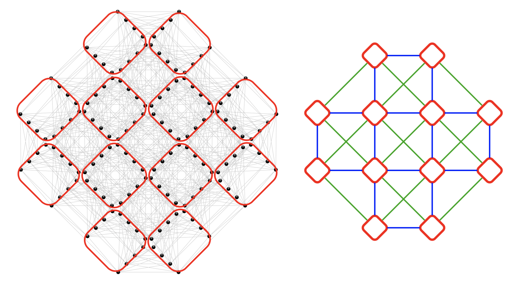
In SpinGlassPEPS.jl solver, a grid of this type can be loaded using the command zephyr_lattice.

SpinGlassPEPS.SpinGlassNetworks.zephyr_lattice — Function

zephyr_lattice(
    size::Tuple{Int64, Int64, Int64}
) -> Dict{Int64, Tuple{Int64, Int64, Int64}}

Create a mapping from Ising graph coordinates to Zephyr lattice coordinates.

This function generates a mapping that relates linear Ising graph coordinates to Zephyr lattice coordinates based on the specified size of the Zephyr lattice in three dimensions: (m, n, t).

Arguments:

size::NTuple{3, Int}: A tuple specifying the size of the Zephyr lattice in three dimensions: (m, n, t), where m is double number of columns, n double number of rows and t denotes number of spins in cluster.

One full Zephyr cluster consists of 16 spins. Convention: t is already divided by 4, so t=4 for Zephyr lattice. E.g. to create 3x3x16 Zephyr lattice, you should use m=6, n=6, t=4.

Returns:

coord_map::Dict: A dictionary that maps Ising graph coordinates to the corresponding Zephyr lattice coordinates.

The zephyr_lattice allows you to build the graph relevant for D-Wave Zephyr architecture.

source

Below you find simple example of usage zephyr_latttice function.

using SpinGlassPEPS

# load instance and create Ising graph
instance = joinpath(
    pkgdir(SpinGlassPEPS),
    "docs", "src", "instances", "zephyr_random", "Z3", "RAU", "001_sg.txt",
)
ig = ising_graph(instance)

# Loaded instance is compatible with Zephyr geometry. Next we create Potts hamiltonian based on Zephyr geometry. 
m = 6
n = 6
t = 4

potts_h = potts_hamiltonian(
    ig,
    cluster_assignment_rule = zephyr_lattice((m, n, t))
)

println("Number of nodes in original instance: ", SpinGlassPEPS.SpinGlassNetworks.nv(ig))